Antibody Fingerprinting
In this Science paper by Georgiev et al. (2013), the authors use a panel of antibody clusters against a panel of virus strains to generate a reference panel of antibody fingerprints that are then used to characterize multiclonal sera. The notation and some clues about recoding their work in R is given below. (Images in this post are best visualized using the Safari browser. Apologies to users on other browsers as I attempt to fix this.)
Antibody Clustering
Stendarting with the antibody clustering analysis (on page 4 of the supplemental), let:
\begin{equation} N_j = \{n_{1j}, n_{2j}, \cdots, n_{ij}, \cdots, n_{vj}\} , \end{equation}
where $N_j$ is the neutralization fingerprint for antibody $j$, and where $n_{ij}$ is the neutralization potency, for which antibody $j$ neutralizes virus strain $i$, and $v$ represents the total number of virus strains. Then, they transform $N_j$ into a rank vector $N_j^R$, where the potency for strain $i$ is replaced by the rank, obtained by sorting the $n_{ij}$ values by potency (highest potency $=1$). For any two given antibodies $j_1$ and $j_2$, the Spearman correlation is calculated for the two rank vectors $N_{j_1}^R$ and $N_{j_2}^R$. To copy their example in R:
na1 <- c(0.5, 0.3, 20.7, 11.3, 13.4)
na2 <- c(0.1, 11.4, 0.1, 0.7, 3.1)
nar1 <- rank(na1)
nar2 <- rank(na2)
cor(nar1, nar2, method="spearman")
[1] -0.4616903
They then use hierarchical clustering in Mathematica. You can cluster using Manhattan distance in R using the following:
d <- dist(as.matrix(mtcars), method="manhattan")
hc <- hclust(d)
plot(hc)
Serum Specificity Delineation
Let $S$ be the set of all virus strains, and let $K$ be the set of antibody clusters:
\begin{equation} S = \{\mathsf{6101.10}, ~~\mathsf{Bal.01}, ~~\cdots, ~~\mathsf{ZM55.28a}\} \end{equation}
\begin{equation} K = \{\mathsf{VRC01-like}, ~~\mathsf{b12-like}, ~~\cdots, \mathsf{10E8-like}\} \end{equation}
For a given cluster $k \in K$, the neutralization fingerprint $R_k$ is defined as:
\begin{equation} R_k = \{\mu_{ik} \left| i \in S \right . \}, \end{equation}
where $\mu_{ik}$ is the median of the ranks for strain $i$ with all antibodies $j$ within antibody cluster $k$. Let $\boldsymbol{R}$ be the matrix of representative neutralization fingerprints for all antibody clusters: $\boldsymbol{R} = \{R_k \left| k \in K \right. \}$, where
\begin{equation} \left[R_{k=1}\right] = \left[\mu_{i=1, k=1} ~~ \mu_{i=2, k=1} ~~ \cdots ~~ \mu_{i=S_T, k=1}\right], \end{equation}
and where $\boldsymbol{R}$ is the reference set of epitope-specific neutralization fingerprints. This is the same as the data in the file neut-rank.csv, and saved as the object abMatrixRanks, where the first column of the .csv gives the strain names $S$ and the first row gives the antibody clusters $K$. Let $v$ be the total number of strains, and $K_T$ be the total number of clusters.
Otherwise represented as:
\begin{equation} \boldsymbol{R} = \left( \begin{array}{cccc} \left[R_{k=1}\right]^T & \left[R_{k=2}\right]^T & \cdots & \left[R_{k=K_T}\right]^T \end{array} \right). \end{equation}
Analagous to the definition ($N_j$) of monoclonal antibody neutralization fingerprinting, let $N_m=\{n_{im} \left| i \in S \right.\}$ be the neutralization pattern for serum $m \in M$, where $M$ represents the set of all sera being tested. You can then transform the serum neutralization pattern $N_m$ into a rank vector $\boldsymbol{D_m}$, based on neutralization / binding potency. Basically, at this point, they want to minimize the residual error between $\boldsymbol{D_m}$ and the neutralization fingerprints $\boldsymbol{R}$ multiplied by some antibody cluster coefficients $\boldsymbol{C_m} = \{c_k^m \left| k \in K \right. \}$.
We want to minimize:
\begin{equation} \parallel \boldsymbol{D_m}-\boldsymbol{R} \cdot \boldsymbol{C_m} \parallel \end{equation}
where we have constrained $\sum_{k \in K} c_k^m =1$, and $0 \leq c_k^m \leq 1$. In our case $R$ is a $\{v \times K_T\}$ matrix, $C_m$ is a $\{K_T \times 1\}$ column vector, and $D_m$ is a $\{1 \times v\}$ row vector, and $\parallel x\parallel$ is the Euclidean or $\ell^2$ norm of $x$: $\parallel x\parallel = \sqrt{x_1^2 + \cdots + x_n^2}$.
We can think of this as a constrained version of the minimization that we perform for ordinary linear regression, without an intercept:
\begin{equation} \parallel \boldsymbol{y}-\boldsymbol{X} \cdot \boldsymbol{\beta} \parallel \end{equation}
Where $\boldsymbol{y}= \boldsymbol{D_m}$, $\boldsymbol{X}=\boldsymbol{R}$, and $\boldsymbol{\beta}=\boldsymbol{C_m}$.
The key words here (to search on Google) are constrained optimization and regression. We can use nnls (non-negative least squares, Lawson-Hanson-flavored). 1 All that is left to do, is to scale the coefficients such that they sum to 1 (divide by the sum of the coefficients).
library("nnls")
A 		<- as.matrix(abMatrixRanks)
b 		<- as.vector(seraFileRanks[,1])
C 		<- nnls(A=A, b=b)
C$x
 [1] 0.00000000 0.00000000 0.00000000 0.30495756 0.05718681 0.11185758
 [7] 0.00000000 0.00000000 0.48295297 0.00000000
sum(C$x)
[1] 0.9569549
C.scaled 	<- C$x/(sum(C$x))
C.scaled
 [1] 0.00000000 0.00000000 0.00000000 0.31867495 0.05975915 0.11688908
 [7] 0.00000000 0.00000000 0.50467683 0.00000000
For instance, performing the calculation on the first row (first serum) would give us:
or
> seraFileRanks[,1]
    6101.1     Bal.01  BG1168.01    CAAN.A2   DU156.12   DU422.01   JRCSF.JB
      17.0       18.0        2.5        7.0       15.0        2.5       20.0
   JRFL.JB KER2018.11     PVO.04    Q168.a2     Q23.17    Q769.h5    RW020.2
      21.0        2.5        5.0        8.0       19.0       13.0        6.0
   THRO.18    TRJO.58     TRO.11     YU2.DG   ZA012.29    ZM106.9   ZM55.28a
       2.5        9.0       16.0       14.0       11.0       10.0       12.0
Here is the final script ab-fp-script.R:
rm(list=ls())
abFile <- read.csv("neut-rank.csv", check.names=FALSE)
seraFile <- read.csv("sera_neut.csv", check.names=FALSE)
abFileSize <- dim(abFile)
seraFileSize <- dim(seraFile)
numAbStrains <- abFileSize[1]
numSeraStrains <- seraFileSize[1]
numAbs <- abFileSize[2]-1
numSera <- seraFileSize[2]-1
abNames <- colnames(abFile)
seraNames <- colnames(seraFile)
## Sort by Strain Name
abFileSorted <- abFile[with(abFile, order(strain)), ]
seraFileSorted <- seraFile[with(seraFile, order(strain)), ]
## Ranks
abMatrixRanks <- abFileSorted[,-1]
seraFileRanks <- apply(X=seraFileSorted[,-1], MARGIN=2, FUN=function(x){rank(-x)})
## Names
abStrainNames <- abFileSorted[,1]
rownames(abMatrixRanks) <- abStrainNames
seraStrainNames <- seraFileSorted[,1]
rownames(seraFileRanks) <- seraStrainNames
if(!(toString(abStrainNames)==toString(seraStrainNames))){
stop("Names do not match in your antibody and strain files.")
}else{
print("Good, your antibody and strain file row names match!")
}
## Perform Minimization (using non-negative least squares)
library("nnls")
find.coefficients <- function(abMatrixRanks, seraFileRanks){
A <- as.matrix(abMatrixRanks)
c.matrix <- matrix(data=NA, nrow=ncol(seraFileRanks),
ncol=ncol(abMatrixRanks))
for(i in 1:ncol(seraFileRanks)){
b <- as.vector(seraFileRanks[,i])
C <- nnls(A=A, b=b)
C.scaled <- C$x/sum(C$x)
c.matrix[i,] <- C.scaled
}
rownames(c.matrix) <- colnames(seraFileRanks)
colnames(c.matrix) <- colnames(abMatrixRanks)
return(c.matrix)
}
coef <- find.coefficients(abMatrixRanks=abMatrixRanks, seraFileRanks=seraFileRanks)
write.csv(coef, "coefficients.csv")
#Alternate, simple heatmap code, without legend
#coef1 <- apply(X=coef, MARGIN=2, FUN=rev)
#heatmap(coef1, Rowv=NA, Colv=NA)
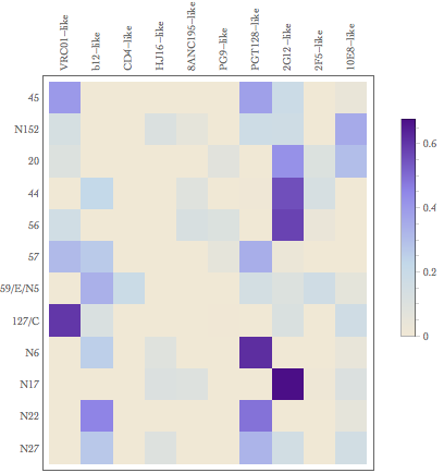
# Plot Heatmap, unclustered
library("gplots")
library("RColorBrewer")
colors <- colorRampPalette(c("beige", "blue"))
lmat = rbind(c(0,3),c(2,1),c(0,4))
lwid = c(1.5,4)
lhei = c(1.5,4,1)
pdf("heatmap1.pdf", width=8, height=8)
heatmap.2(coef, dendrogram="none", col=colors, trace="none",
scale="none", margins=c(8,5), Rowv=FALSE, Colv=FALSE,
lmat=lmat, lwid=lwid, lhei=lhei, density.info="none")
dev.off()
pdf("stackedbars.pdf", width=12, height=6)
colors <- rainbow(length(colnames(coef)))
barplot(t(coef), col=colors, xlim=c(0,length(colnames(coef))*2))
legend("topright", legend=colnames(coef), fill=colors)
dev.off()Result from original Mathematica vs.
Result from my R script

Alternative visualization using stacked bars

-
(Alternative options may exist with the
optimorconstrOptimfunctions in theRpackagestats.) ↩